ReLU Fields: The Little Non-linearity That Could

Abstract

In many recent works, multi-layer perceptions (MLPs) have been shown to be suitable for modeling complex spatially-varying functions including images and 3D scenes. Although the MLPs are able to represent complex scenes with unprecedented quality and memory footprint, this expressive power of the MLPs, however, comes at the cost of long training and inference times. On the other hand, bilinear/trilinear interpolation on regular grid based representations can give fast training and inference times, but cannot match the quality of MLPs without requiring significant additional memory. Hence, in this work, we investigate what is the smallest change to grid-based representations that allows for retaining the high fidelity result of MLPs while enabling fast reconstruction and rendering times. We introduce a surprisingly simple change that achieves this task – simply allowing a fixed non-linearity (ReLU) on interpolated grid values. When combined with coarse to-fine optimization, we show that such an approach becomes competitive with the state-of-the-art. We report results on radiance fields, and occupancy fields, and compare against multiple existing alternatives.

ReLU-Fields

In this work, we present the following contributions:

we propose a minimal extension to grid-based signal representations, which we refer to as ReLU Fields.
we show that this representation is simple, does not require any neural networks, is directly differentiable (and hence easy to optimize), and is fast to optimize and evaluate (i.e. render).
we empirically validate our claims by showing applications where ReLU Fields plug in naturally: first, image-based 3D scene reconstruction; and second, implicit modeling of 3D geometries.

Method explanation

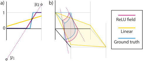
Representing a ground-truth function (blue) in a 1D (a) and 2D (b) grid cell using the linear basis (yellow) and a ReLUField (pink). The reference has a c1-discontinuity inside the domain that a linear basis cannot capture. A ReLUField will pick two values $y_{1}$ and $y_{2}$ , such that their interpolation, after clamping will match the sharp c1-discontinuity in the ground-truth (blue) function. Please note that a hard-clip at max 1 is also needed usually for rendering as is done in both the examples shown here.

It's just a little ReLU

We look for a representation of $n$ -valued signals on an $m$ -dimensional coordinate domain $R^{m}$ . For simplicity, we explain the method for $m = 3$ . Our representation is strikingly simple. We consider a regular ( $m = 3$ )-dimensional ( $r \times r \times r$ )-grid $G$ composed of $r$ voxels along each side. Each voxel has a certain size defined by its diagonal norm in the ( $m = 3$ )-dimensional space and holds an $n$ -dimensional vector at each of its ( $2^{m = 3} = 8$ ) vertices. Importantly, even though they have matching number of dimensions, these values do not have a direct physical interpretation (e.g. color, density, or occupancy), which always have some explicitly-defined range, e.g. $[0, 1]$ or $[0, + \infty)$ . Rather, we store unbounded values on the grid; and thus for technical correctness, we call these grids "feature"-grids instead of signal-grids. The features at grid vertices are then interpolated using $m = 3$ -linear (trilinear) interpolation, and followed by a single non-linearity: the $R e L U$ function, i.e. $ReLU (x) = max (0, x)$ which maps negative input values to 0 and all other values to themselves. Note that this approach does not have any MLP or other neural-network that interprets the features, instead they are simply clipped before rendering. Intuitively, during optimization, these feature-values at the vertices can go up or down such that the ReLU clipping plane best aligns with the c1-discontinuities within the ground-truth signal. Above figure illustrates this concept.

Experimental evaluation

2D Pixel Fields didactic example

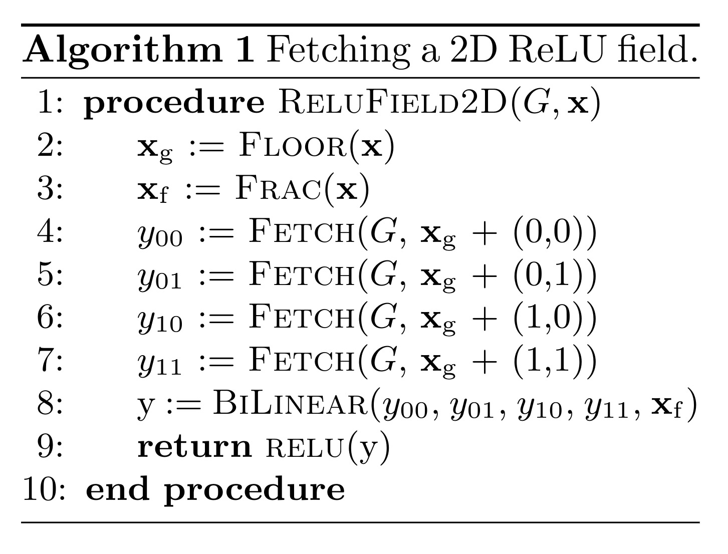
As a didactic example, we fit an image into a 2D ReLU-Field grid similar to SIREN, where grid values are stored as floats in the $(- \infty, + \infty)$ range. For any query position, we interpolate the grid values before passing through the ReLU function (see Algorithm above). Since the image-signal values are expected to be in the $[0, 1]$ range, we apply a hard-upper-clip on the interpolated values just after applying the ReLU. We can see in adjoining figure that ReLUFields allows us to represent sharp edges at a higher fidelity than bilinear interpolation (without the ReLU) at the same resolution grid size. One limitation of this representation is that it can only well represent signals that have sparse c1-discontinuities, such as this flat-shaded images and as we show later, 3D volumetric density. However, other types of signals, such as natural images, do not benefit from using our proposed representation.

3D Occupancy Fields

Quantitative Scores (volumetric-IoU)

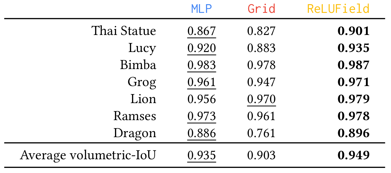
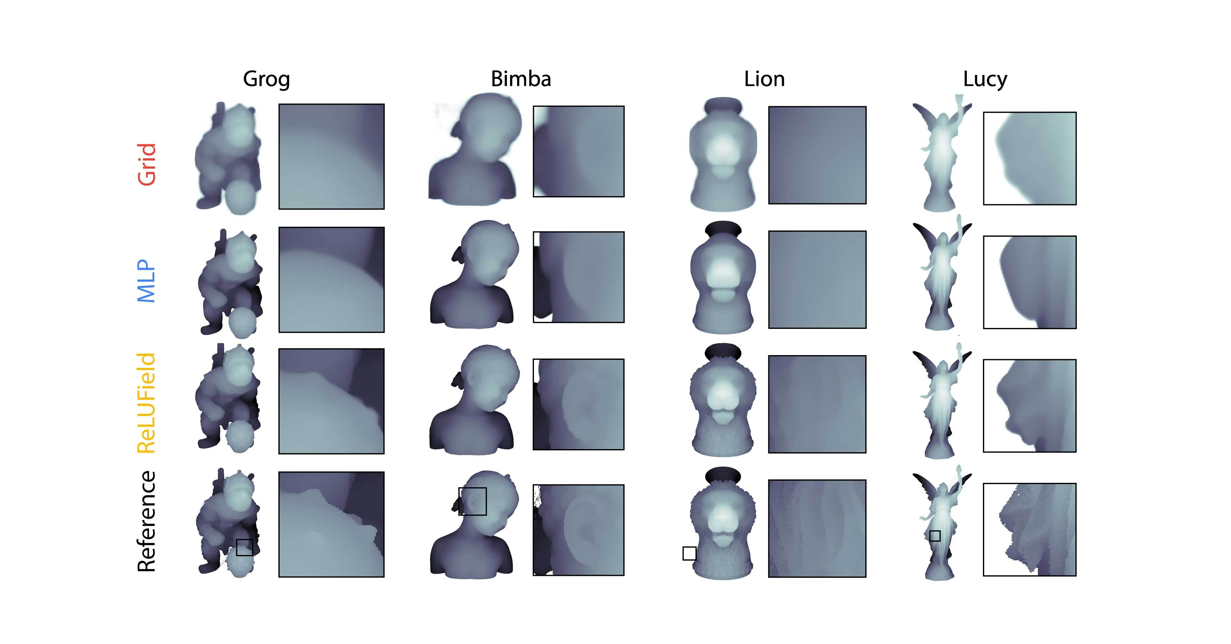
Evaluation results on modeling 3D geometries as occupancy fields. Metric used is Volumetric-IoU. The baseline MLP is our implementation of OccupancyNetworks.

3D occupancy field qualitative results

3D Radiance Fields

Quantitative Scores (PSNR & LPIPS)

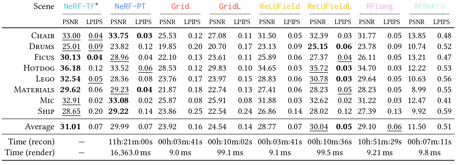
Evaluation results on 3D synthetic scenes. Metrics used are PSNR (↑) / LPIPS (↓). The column NeRF-TF^* quotes PSNR values from prior work, and as such we do not have a comparable runtime for this method.

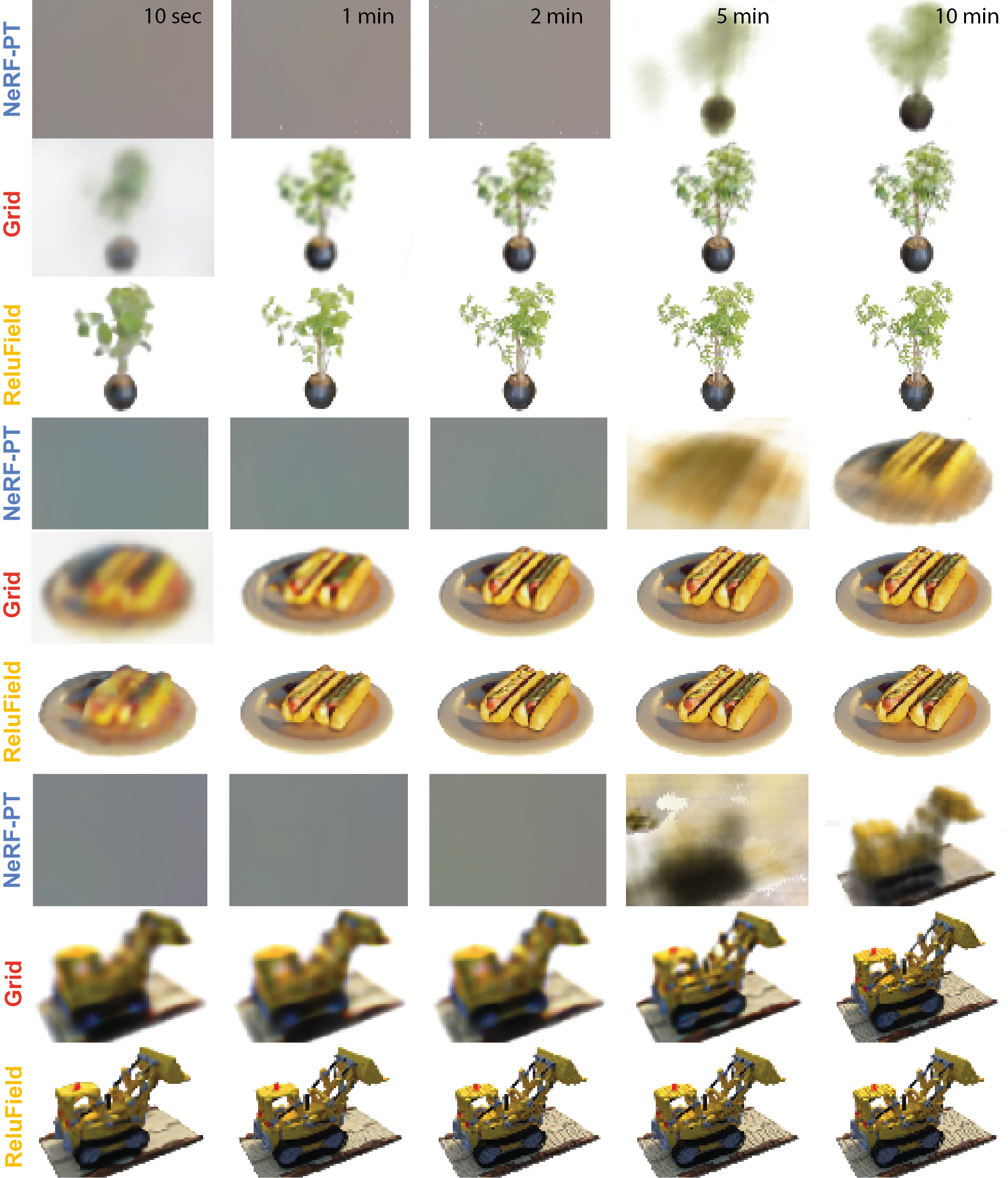
Training timelapse (Figure version)

Qualitative comparison between NeRF-PT, Grid and ReLUField . Grid-based versions converge much faster, and we can see significant sharpness improvements of ReLUField over Grid , for example in the leaves of the plant.

Training timelapse (video-loop version)

Spiral path ReLU-Fields results

360-degree comparison results

Bibtex


    @inproceedings{
      ReluField_sigg_22,
      author = {Karnewar, Animesh and Ritschel, Tobias and Wang, Oliver and Mitra, Niloy},
      title = {ReLU Fields: The Little Non-Linearity That Could},
      year = {2022},
      isbn = {9781450393379},
      publisher = {Association for Computing Machinery},
      address = {New York, NY, USA},
      url = {https://doi.org/10.1145/3528233.3530707},
      doi = {10.1145/3528233.3530707},
      booktitle = {ACM SIGGRAPH 2022 Conference Proceedings},
      articleno = {27},
      numpages = {9},
      keywords = {spatial representations, volume rendering,
                  neural representations, regular data structures},
      location = {Vancouver, BC, Canada},
      series = {SIGGRAPH '22}
    }

Acknowledgements

The research was partially supported by the European Union’s Horizon 2020 research and innovation programme under the Marie Skłodowska-Curie grant agreement No. 956585, gifts from Adobe, and the UCL AI Centre.

This project-web-page has been built using the super-cool HyperNeRF's project-webpage as a template.